Calculate Johnson-Neyman intervals for 2-way interactions

johnson_neyman finds so-called "Johnson-Neyman" intervals for understanding where simple slopes are significant in the context of interactions in multiple linear regression.

Usage

johnson_neyman(
  model,
  pred,
  modx,
  vmat = NULL,
  alpha = 0.05,
  plot = TRUE,
  control.fdr = FALSE,
  line.thickness = 0.5,
  df = "residual",
  digits = getOption("jtools-digits", 2),
  critical.t = NULL,
  sig.color = "#00BFC4",
  insig.color = "#F8766D",
  mod.range = NULL,
  title = "Johnson-Neyman plot",
  y.label = NULL,
  modx.label = NULL
)

Arguments

model: A regression model. It is tested with lm, glm, and svyglm objects, but others may work as well. It should contain the interaction of interest. Be aware that just because the computations work, this does not necessarily mean the procedure is appropriate for the type of model you have.
pred: The predictor variable involved in the interaction.
modx: The moderator variable involved in the interaction.
vmat: Optional. You may supply the variance-covariance matrix of the coefficients yourself. This is useful if you are using robust standard errors, as you could if using the sandwich package.
alpha: The alpha level. By default, the standard 0.05.
plot: Should a plot of the results be printed? Default is TRUE. The ggplot2 object is returned either way.
control.fdr: Logical. Use the procedure described in Esarey & Sumner (2017) to limit the false discovery rate? Default is FALSE. See details for more on this method.
line.thickness: How thick should the predicted line be? This is passed to geom_path as the size argument, but because of the way the line is created, you cannot use geom_path to modify the output plot yourself.
df: How should the degrees of freedom be calculated for the critical test statistic? Previous versions used the large sample approximation; if alpha was .05, the critical test statistic was 1.96 regardless of sample size and model complexity. The default is now "residual", meaning the same degrees of freedom used to calculate p values for regression coefficients. You may instead choose any number or "normal", which reverts to the previous behavior. The argument is not used if control.fdr = TRUE.
digits: An integer specifying the number of digits past the decimal to report in the output. Default is 2. You can change the default number of digits for all jtools functions with options("jtools-digits" = digits) where digits is the desired number.
critical.t: If you want to provide the critical test statistic instead relying on a normal or t approximation, or the control.fdr calculation, you can give that value here. This allows you to use other methods for calculating it.
sig.color: Sets the color for areas of the Johnson-Neyman plot where the slope of the moderator is significant at the specified level. "black" can be a good choice for greyscale publishing.
insig.color: Sets the color for areas of the Johnson-Neyman plot where the slope of the moderator is insignificant at the specified level. "grey" can be a good choice for greyscale publishing.
mod.range: The range of values of the moderator (the x-axis) to plot. By default, this goes from one standard deviation below the observed range to one standard deviation above the observed range and the observed range is highlighted on the plot. You could instead choose to provide the actual observed minimum and maximum, in which case the range of the observed data is not highlighted in the plot. Provide the range as a vector, e.g., c(0, 10).
title: The plot title. "Johnson-Neyman plot" by default.
y.label: If you prefer to override the automatic labelling of the y axis, you can specify your own label here. The y axis represents a slope so it is recommended that you do not simply give the name of the predictor variable but instead make clear that it is a slope. By default, "Slope of [pred]" is used (with whatever pred is).
modx.label: If you prefer to override the automatic labelling of the x axis, you can specify your own label here. By default, the name modx is used.

Value

bounds: The two numbers that make up the interval.
cbands: A dataframe with predicted values of the predictor's slope and lower/upper bounds of confidence bands if you would like to make your own plots
plot: The ggplot object used for plotting. You can tweak the plot like you could any other from ggplot.

Details

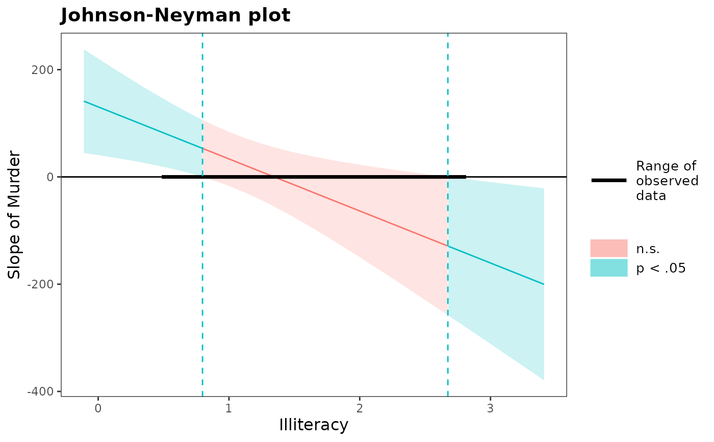
The interpretation of the values given by this function is important and not always immediately intuitive. For an interaction between a predictor variable and moderator variable, it is often the case that the slope of the predictor is statistically significant at only some values of the moderator. For example, perhaps the effect of your predictor is only significant when the moderator is set at some high value.

The Johnson-Neyman interval provides the two values of the moderator at which the slope of the predictor goes from non-significant to significant. Usually, the predictor's slope is only significant outside of the range given by the function. The output of this function will make it clear either way.

One weakness of this method of probing interactions is that it is analogous to making multiple comparisons without any adjustment to the alpha level. Esarey & Sumner (2017) proposed a method for addressing this, which is implemented in the interactionTest package. This function implements that procedure with modifications to the interactionTest code (that package is not required to use this function). If you set control.fdr = TRUE, an alternative t statistic will be calculated based on your specified alpha level and the data. This will always be a more conservative test than when control.fdr = FALSE. The printed output will report the calculated critical t statistic.

This technique is not easily ported to 3-way interaction contexts. You could, however, look at the J-N interval at two different levels of a second moderator. This does forgo a benefit of the J-N technique, which is not having to pick arbitrary points. If you want to do this, just use the sim_slopes function's ability to handle 3-way interactions and request Johnson-Neyman intervals for each.

References

Bauer, D. J., & Curran, P. J. (2005). Probing interactions in fixed and multilevel regression: Inferential and graphical techniques. Multivariate Behavioral Research, 40(3), 373-400. doi:10.1207/s15327906mbr4003_5

Esarey, J., & Sumner, J. L. (2017). Marginal effects in interaction models: Determining and controlling the false positive rate. Comparative Political Studies, 1–33. Advance online publication. doi:10.1177/0010414017730080

Johnson, P.O. & Fay, L.C. (1950). The Johnson-Neyman technique, its theory and application. Psychometrika, 15, 349-367. doi:10.1007/BF02288864

Author

Jacob Long jacob.long@sc.edu

Examples

# Using a fitted lm model
states <- as.data.frame(state.x77)
states$HSGrad <- states$`HS Grad`
fit <- lm(Income ~ HSGrad + Murder*Illiteracy,
  data = states)
johnson_neyman(model = fit, pred = Murder,
  modx = Illiteracy)
#> JOHNSON-NEYMAN INTERVAL
#> 
#> When Illiteracy is OUTSIDE the interval [0.80, 2.67], the slope of
#> Murder is p < .05.
#> 
#> Note: The range of observed values of Illiteracy is [0.50, 2.80]
#>